Measuring and Visualizing Domain Specific Word Use
(Work in progress)
Goals and approach
Language adapts to the communicative needs of its context, along dimensions such as domain, register, and time. This is reflected in preferential choices of vocabulary, grammar, meaning, and style, which differentiate language use by context. This visualization aims at exploring domain specific word use based on three related but complementary measures:
- Typicality of a word measures how typical a word is for a domain compared to other domains. Informally, if a word is significantly more frequent in a domain, it is typical for the domain [1].
- (Paradigmatic) Productivity of a word measures how many (paradigmatically) similar words are used in the domain. A word w with a paradigmatic neighbourhood (semantic field) consisting of many words is considered highly productive [2].
- Ambiguity of a word measures how different its use in one domain is from another. Formally, this is defined as the cosine distance between the domain specific embeddings of a word [3].
Productivity and Ambiguity require a representation of word use in a domain. To this end, we use word embeddings (Mikolov et al. 2013), which have become a popular means to analyze the semantics of words based on their actual use in large corpora. The main idea of word embeddings is to reduce the very high dimensionality of word co-occurrence contexts, the size of the vocabulary, to few dimensions, such as 100-200. For the word embeddings used in this visualization, we employ the structured skip gram approach by Ling et al. (2015), using a one-hot encoding for words as input layer, a 200 dimensional hidden layer, and a positional one-hot encoding for the context words in a window of [-5,5] as the output layer. This approach takes word order into account, and thus also captures syntactic regularities of word use.
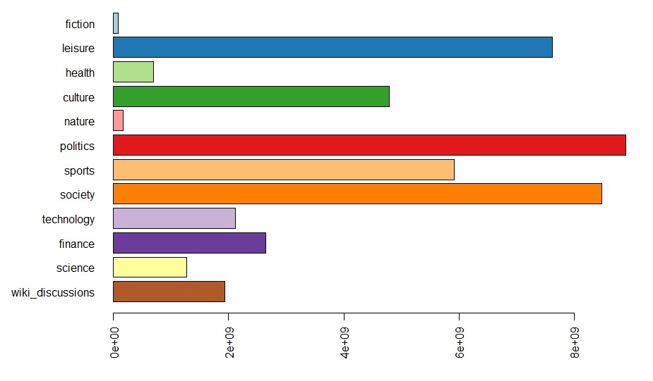
As base corpus, we use the DeReKo-2017-II edition of the German Reference Corpus (Institut für Deutsche Sprache 2017; Kupietz et al 2010, 2018) containing 33 billion tokens. For the separation into domains, we use 11 of the top-level domain categories annotated in the metadata of DeReKo texts (Weiss 2005) and Wikipedia discussions (ref). The individual domains contain between 80 million and 9 billion tokens (see Figure 1).
For deriving domain specific word embeddings we adapt the approach of Dubossarsky et al. (2015), Fankhauser and Kupietz (2017), there used for diachronic corpora (see also Diachronic Visualization). We first compute embeddings for the base corpus and use them to initialize training of domain specific embeddings. Thereby the embeddings are comparable between individual domains and the base corpus. On this basis the paradigmatic neighbourhood of words with similar meanings is defined by the cosine similarity of their embeddings. To visualize the embeddings we further reduce their 200 dimension to two dimensions using t-distributed stochastic neighbourhood embedding (Van der Maaten & Hinton 2008).
A quick guide
The visualization consists of three main areas:
To the left, a bubble chart represents the color encoded semantic space of words, with the size of bubbles proportional to the square root of the relative frequency in the chosen domain, and the color indicating the domain of a word. Words with similar use typically are positioned closely to each other.
The top right provides a heatmap representing the overall distance between the individual domains, formalized as the Kullback Leibler Divergence of their unigram language models, ranging from deep red for a large distance (Fiction, Sports, Wikipedia Discussions) to yellow for a small distance. The heatmap doubles as a selector for choosing a pair of domains to compare with each other, the main diagonal serves for comparing a domain with the base corpus. Clicking on the title DeReKo Domains chooses the (initial) overall comparison of the most typical words for each domain with the base corpus.
The top right also provides a number of visualization options.
- +/- zooms the visualization in and out as an alternative to zooming with the scroll wheel.
- ? brings up this page.
- Zoom By chooses between different ways to determine which words are shown on different zoom levels (ranging from 0 to 14). With freq clst and kld clst zoom levels are computed by partitioning the words into an increasing number of clusters (from 200 to 23.000) and assigning only the most frequent (freq clst) or most typical (kld clst) word of each cluster to a zoom level. This approach distributes the bubbles rather evenly in the semantic space. In contrast, freq and kld simply associate the top 200 words to the first zoom level and so on. This leads to more unevenly distributed bubbles, but shows more clearly which regions are mainly populated by a domain.
- Color toggles between coloring the bubbles with a qualitative vs. divergent color scheme.
- Domain toggles between displaying both domains or only one domain in the bubble chart.
- Show allows to hide words, excluded ne (named entities), and/or bubbles from the bubble chart.
- Exclude allows to exclude various kinds of named entities and english words from the comparison word lists (see below). This is mainly for convenience, as named entities, comprising over 18% of the types and over 6% of the tokens often stand out w.r.t. all measures of domain specific word use, and thus make it difficult to focus on linguistically more interesting cases. Note that this feature is currently not based on proper named entity recognition, but rather on a (precision minded) post hoc annotation of domain specific word embedding clusters.
The bottom right provides a comparison word list for the chosen pair of domains, with the following columns:
- word gives the word.
- fpm its frequency per million in the first domain.
- kld its typicality in comparison to the second domain.
- ent its paradigmatic productivity in the first domain.
- entd the difference between productivity in the first domain and the second domain.
- dist the cosine distance between the two domain specific domain embeddings, multiplied by the sign of its typicality, such that words with negative distances are distant and typical for the second domain.
- dist2d the eukledian distance between the two domain specific 2D positions. While dist2d is of course less accurate than dist, sorting descending by dist2d allows to identify (ambigous) words whose paradigmatic neighbourhoods are still rather clearly distinguished in the 2D visualization.
The word list can be sorted on all columns, searched for words, and filtered by giving lower bounds. Filtering is in particular useful to focus on words with a minimum frequency per million, or on words typical for a domain (kld > 0). Clicking on a word zooms and centers the bubble chart on its position in the first domain, a double click selects its position in the second domain. This allows to quickly inspect its different meanings by its paradigmatic neighbours.
Available visualizations
The following visualizations are currently available:
- DeReKo with its 11 top level domains. (Perplexity for tsne: 30)
- DeReKo with Wikipedia Discussions and the 11 top level domains. (Perplexity for tsne: 30)
- DeReKo with Wikipedia Discussions and the 11 top level domains. (Perplexity for tsne: 100)
- DeReKo with Wikipedia Discussions and the 11 top level domains. (Perplexity for tsne: 200)
The tsne hyperparameter Perplexity determines roughly how well local neighbourhoods are preserved in two dimensions. Perplexities 100 and 200 seem to work better than 30. Note that the visualization takes some time to load (depending on your connection between 10 and 60 seconds).
Some example analysis
Macro Analysis
To illustrate the introduced measures and their interaction, we start with a macro analytic perspective:
Figure 2(a) shows how specific word use is in the indivual domains by means of the Jensen-Shannon divergence between their (unigram) language models. Red means high divergence, yellow means low. We can see that fiction (FI), sports (SP), and wikipedia discussions (WD) stand out with rather specific word distributions, and thus (reddish) high divergence, whereas, e.g., politics (PO) and society (SG) are rather close.
| FI | FR | GE | KU | NU | PO | SP | SG | TI | WF | WI | WD | |
|---|---|---|---|---|---|---|---|---|---|---|---|---|
| FI | 0.00 | 0.32 | 0.32 | 0.23 | 0.29 | 0.29 | 0.36 | 0.21 | 0.36 | 0.39 | 0.30 | 0.33 |
| FR | 0.32 | 0.00 | 0.16 | 0.11 | 0.16 | 0.13 | 0.21 | 0.11 | 0.14 | 0.20 | 0.14 | 0.36 |
| GE | 0.32 | 0.16 | 0.00 | 0.20 | 0.16 | 0.13 | 0.27 | 0.11 | 0.15 | 0.16 | 0.09 | 0.31 |
| KU | 0.23 | 0.11 | 0.20 | 0.00 | 0.21 | 0.15 | 0.22 | 0.12 | 0.21 | 0.23 | 0.16 | 0.30 |
| NU | 0.29 | 0.16 | 0.16 | 0.21 | 0.00 | 0.19 | 0.27 | 0.15 | 0.18 | 0.25 | 0.15 | 0.36 |
| PO | 0.29 | 0.13 | 0.13 | 0.15 | 0.19 | 0.00 | 0.23 | 0.08 | 0.13 | 0.11 | 0.12 | 0.27 |
| SP | 0.36 | 0.21 | 0.27 | 0.22 | 0.27 | 0.23 | 0.00 | 0.21 | 0.25 | 0.26 | 0.26 | 0.37 |
| SG | 0.21 | 0.11 | 0.11 | 0.12 | 0.15 | 0.08 | 0.21 | 0.00 | 0.14 | 0.16 | 0.13 | 0.22 |
| TI | 0.36 | 0.14 | 0.15 | 0.21 | 0.18 | 0.13 | 0.25 | 0.14 | 0.00 | 0.16 | 0.13 | 0.36 |
| WF | 0.39 | 0.20 | 0.16 | 0.23 | 0.25 | 0.11 | 0.26 | 0.16 | 0.16 | 0.00 | 0.15 | 0.31 |
| WI | 0.30 | 0.14 | 0.09 | 0.16 | 0.15 | 0.12 | 0.26 | 0.13 | 0.13 | 0.15 | 0.00 | 0.28 |
| WD | 0.33 | 0.36 | 0.31 | 0.30 | 0.36 | 0.27 | 0.37 | 0.22 | 0.36 | 0.31 | 0.28 | 0.00 |
| FI | FR | GE | KU | NU | PO | SP | SG | TI | WF | WI | WD | |
|---|---|---|---|---|---|---|---|---|---|---|---|---|
| FI | 92.0 | 0.7 | 0.2 | 2.0 | 0.3 | 0.6 | 0.2 | 1.6 | 0.1 | 0.6 | 0.5 | 1.0 |
| FR | 0.1 | 87.1 | 0.6 | 3.7 | 0.4 | 1.7 | 1.7 | 1.3 | 1.5 | 0.8 | 1.0 | 0.1 |
| GE | 0.1 | 2.0 | 83.6 | 0.4 | 1.0 | 3.0 | 0.2 | 2.1 | 1.3 | 3.1 | 2.4 | 0.9 |
| KU | 0.5 | 4.9 | 0.1 | 89.5 | 0.1 | 1.1 | 1.0 | 1.2 | 0.1 | 0.4 | 0.6 | 0.6 |
| NU | 0.5 | 2.2 | 1.8 | 0.2 | 89.7 | 0.4 | 0.6 | 0.6 | 1.6 | 0.3 | 1.9 | 0.1 |
| PO | 0.1 | 1.8 | 1.0 | 1.0 | 0.1 | 87.1 | 0.5 | 1.8 | 0.7 | 4.3 | 0.7 | 1.0 |
| SP | 0.0 | 1.2 | 0.1 | 0.5 | 0.0 | 0.5 | 96.9 | 0.2 | 0.1 | 0.3 | 0.0 | 0.1 |
| SG | 0.9 | 2.8 | 1.9 | 3.4 | 0.4 | 3.7 | 0.7 | 81.9 | 1.8 | 1.3 | 0.1 | 1.3 |
| TI | 0.0 | 1.9 | 0.9 | 0.2 | 0.4 | 1.8 | 0.4 | 1.3 | 88.4 | 2.4 | 1.6 | 0.6 |
| WF | 0.1 | 0.6 | 1.3 | 0.6 | 0.0 | 5.4 | 0.6 | 0.9 | 1.6 | 85.1 | 2.3 | 1.5 |
| WI | 0.4 | 1.4 | 1.9 | 1.1 | 1.1 | 1.1 | 0.0 | 0.2 | 2.5 | 2.7 | 86.5 | 1.2 |
| WD | 0.6 | 0.4 | 0.6 | 1.4 | 0.0 | 2.2 | 0.2 | 1.0 | 0.8 | 2.6 | 1.5 | 88.8 |
Figure 2(b) illustrates that paradigmatically related words are often typical for the same domain. Each cell at position Domain y/Domain x gives the probability (*100) that the nearest neighbour of a word typical for Domain y (with maximum cosine distance 0.3) is typical for Domain x. Overall, there is a 89% chance that the nearest neighbour is typical for the same domain (main diagonal). For fiction and sports the chance is even 92% and 97%, their typical words thus form the most tightly knit paradigmatic clusters.
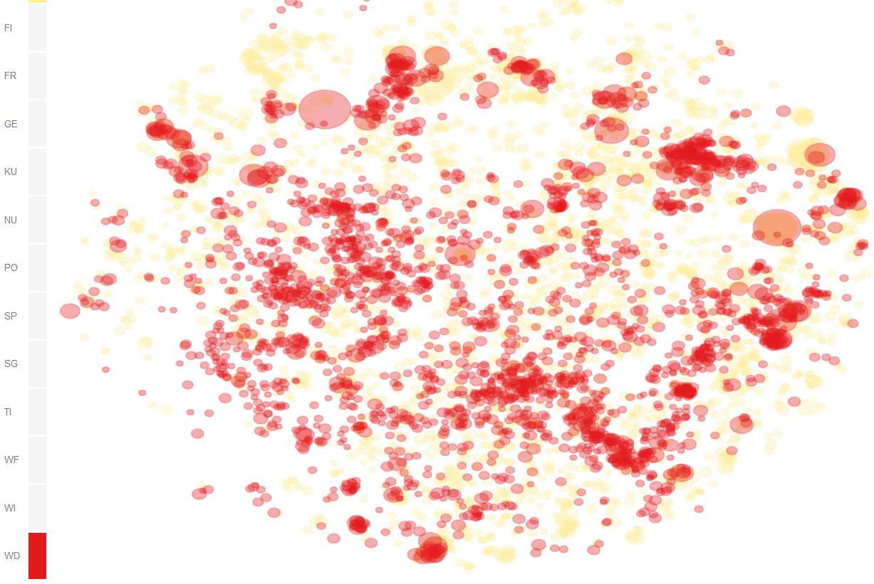
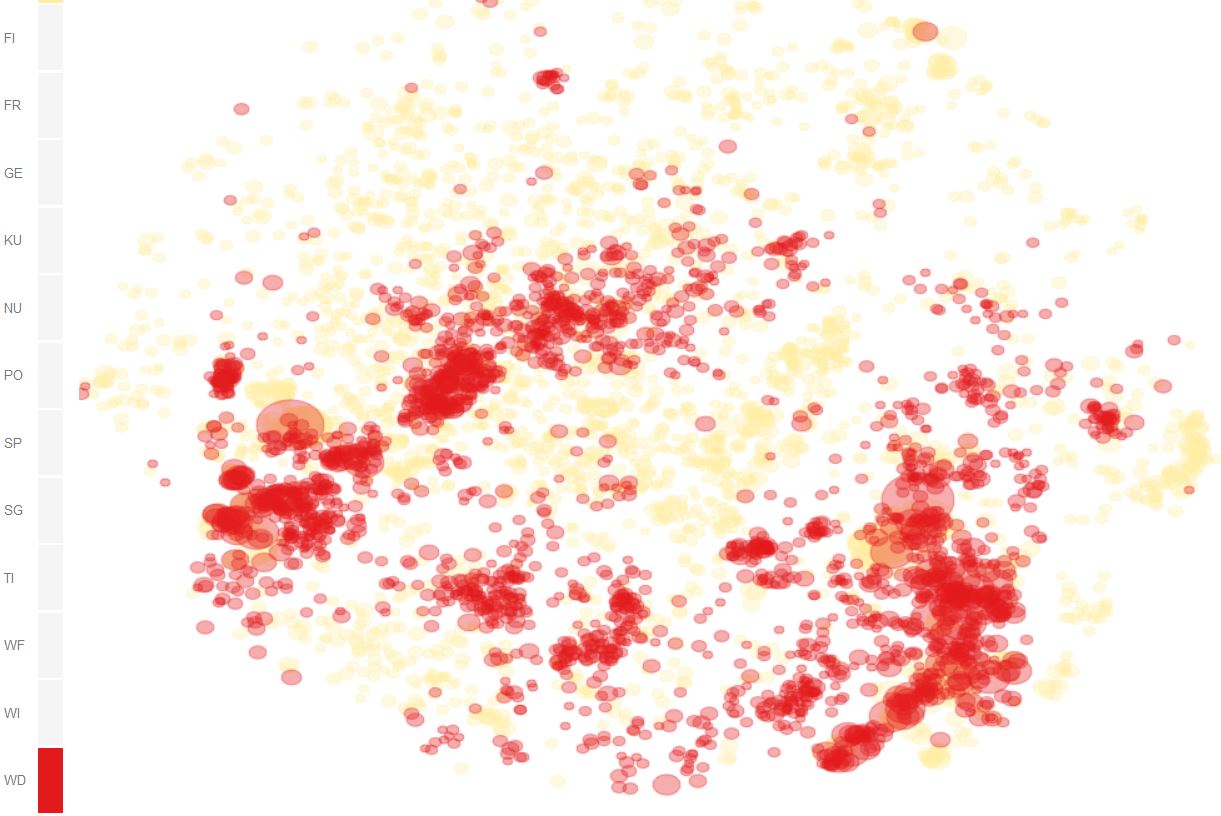
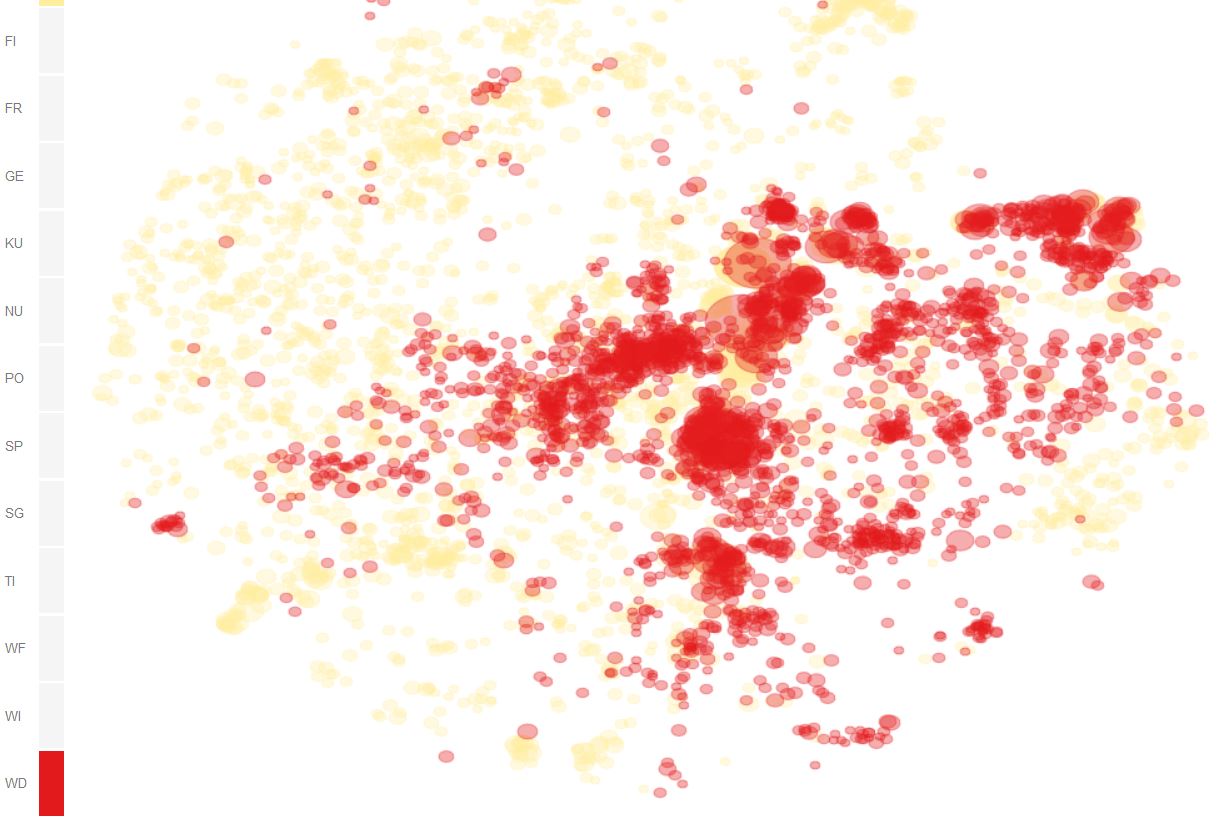
Figure 3 provides a more indepth perspective on domain specific paradigmatic clusters by visually correlating domain (color) with semantics (position in 2D) of words. Especially for perplexities 100 and 200, which preserve local neighbourhoods fairly well, we can see that words typical for wikipedia discussions (red) populate rather specific regions, whereas words in the base corpus DeReKo (yellow) populate the entire semantic space [4].
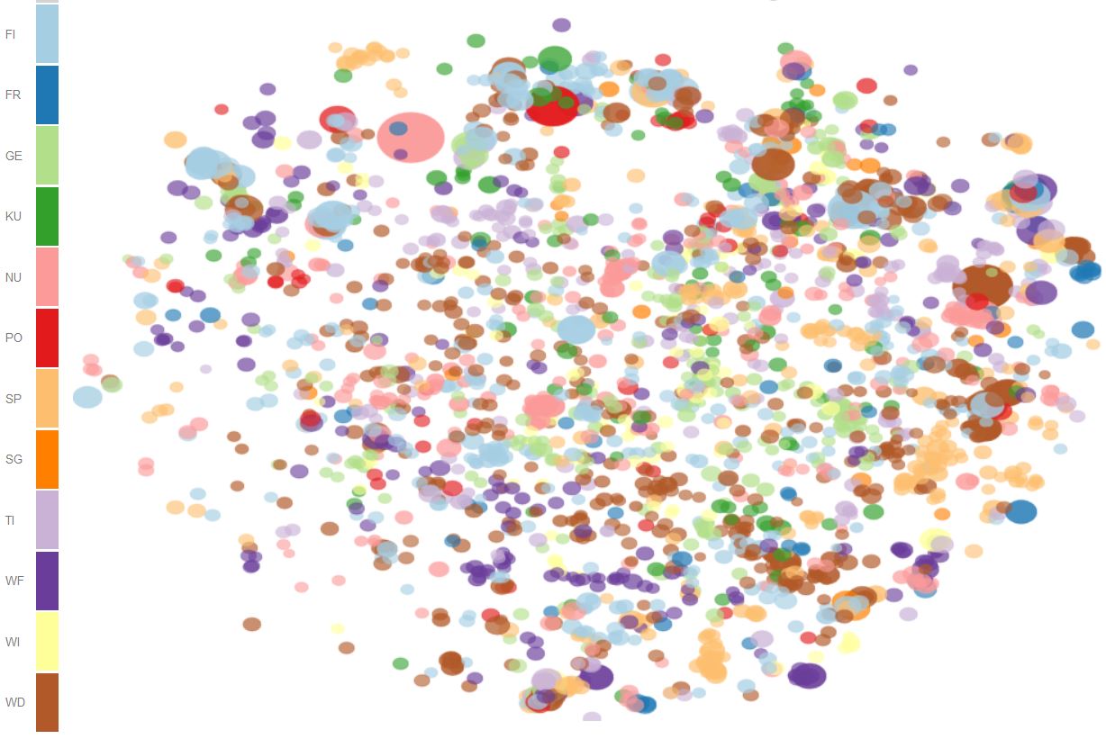
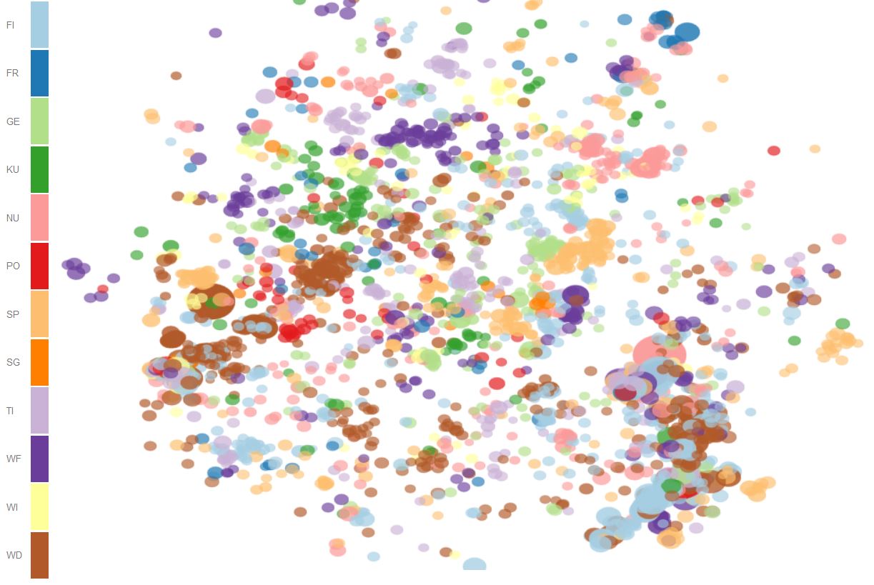
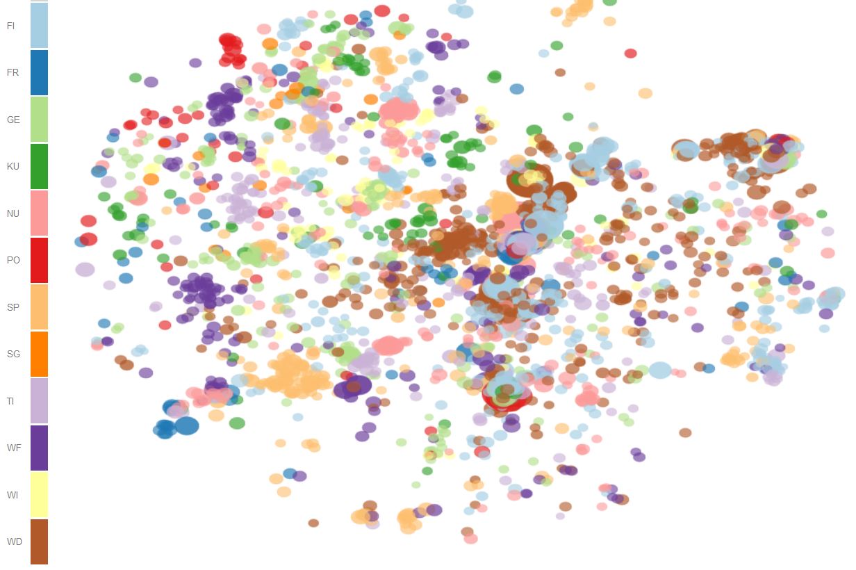
Figure 4 shows the 2D distribution of the most typical words for all domains at various perplexities. Again, especially for higher perplexities, we can clearly identify clusters of paradigmatically related words typical for the same domain.
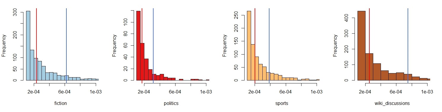
Finally, Figures 5-7 show the distributions of the individual measures for selected domains. Figure 5 shows the distributions of individual KLD values (typicality) > 0.001, words with smaller and negative KLD values constitute the majority, but do not contribute to typicality. Mean (blue) and median (red) of the domains with distinctive language models fiction, sport, wikipedia discussions are significantly larger than for domains closer to the base corpus, such as politics.
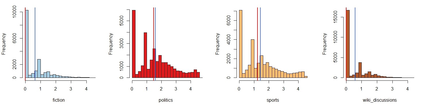
Figure 6 shows the distributions of the individual entropies (paradigmatic productivity). These show an opposite trend. On average, the domains fiction and wikipedia discussions have lower paradigmatic productivity (mean and even more strikingly median). One reason for this may be the technical setup: We currently only consider the most frequent 30.000 words in the base corpus DeReKo, and the language models of these two domains are rather distinct. Thus, some domain specific pardigmatic neighbours may not be included in the overall top 30.000, causing artificially low entropies for some domain specific words which are in the top 30.000. However, sports has a rather distinct language model too, but displays rather high productivity. This requires further careful analysis. Figure 7 shows means and medians of the paradigmatic productivities for all domains. In addition, the distributions are not as smooth as the distributions for kld and distance, but contain gaps, especially on the low end. This is most likely due to the somewhat arbitrary cut-off at maximum cosine-distance 0.3, which causes many words to have no neighbours, and thus entropy 0. However, on the higher end, the distributions are fairly smooth.
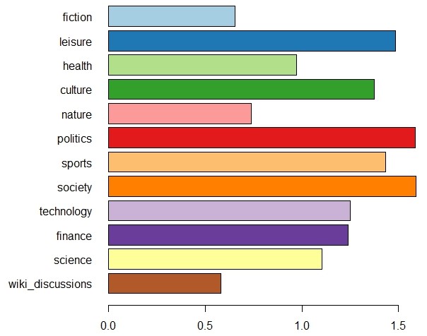
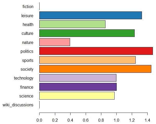
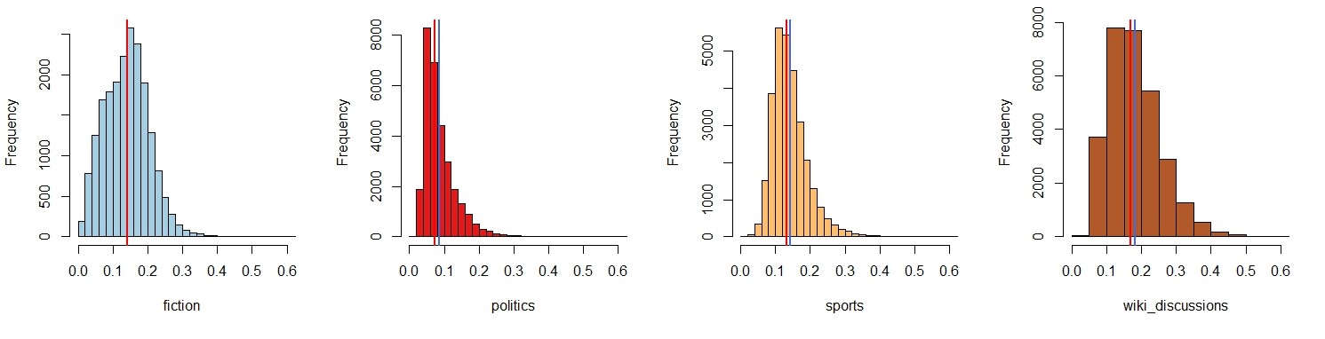
Figure 8 shows the distributions of the cosine-distances (ambiguity). On average, these show a similar trend as the kld distributions, i.e., domains with specific unigram language models (kld), e.g., fiction and wikipedia discussions also have a higher mean and median distance. We can see that the domain specific training regime leads to a small but general meaning shift, i.e., there are rather few words which do not change their meaning at all.
Micro Analysis
Table 1 displays the top 10 words by kld (typicality) for selected domains in comparison to the base corpus. Just 10 words can of course not sufficiently characterize a domain, but still the largerly interpersonal discourse in fiction and wikipedia discussions is hinted at by personal pronouns, the nominal style of politics and science by definite articles and passive (werden), and the main themes of culture and sports by according thematic words.
| fiction | culture | politics | sports | science | discussions |
|---|---|---|---|---|---|
| ich | </s> | </s> | <num> | </s> | <num> |
| daß | und | die | </s> | werden | du |
| </s> | er | der | gegen | die | ich |
| er | Musik | dass | den | sind | Artikel |
| sie | von | für | Trainer | oder | nicht |
| du | mit | werden | Spiel | Forscher | </s> |
| und | als | nicht | Mannschaft | ist | Du |
| mir | Film | sei | Sieg | von | Ich |
| mich | Publikum | des | Saison | Wissenschaftler | ist |
| so | Band | Stadt | Platz | etwa | Wikipedia |
Table 2 gives the top 10 words by their domain specific paradigmatic productivity, discarding non typical words with negative kld. fiction contains an assortment of past tense and modal words, some adverbial connectors, and some numerals, which, like named entities are of course inherently productive. wikipedia discussions lists a larger variety of adverbial connectors together with adjectives expressing criticism. culture contains mainly judgemental adjectives with clearly positive sentiment, whereas politics leans towards judgemental adjectives with predominantly negative sentiment. sports also contains some adjectives with positive sentiment, together with other entries with rather low kld with less obvious relationship to sports. In science the inherently productive field of color adjectives appears on top. As mentioned above, the paradigmatic neighbourhoods of named entities are typically very productive, and are thus excluded in Table 2.
| fiction | culture | politics | sports | science | discussions |
|---|---|---|---|---|---|
| Gleichwohl | mitreißenden | absurd | enzyklopädisch | rosa | fragwürdig |
| Überdies | humorvollen | inakzeptabel | sensationellen | orange | Nichtsdestotrotz |
| sollte | stimmungsvollen | kontraproduktiv | bemerkenswerten | Energie- | Jedenfalls |
| würde | eindrucksvollen | abwegig | Formulierung | Bohnen | problematisch |
| zog | fantastischen | ärgerlich | eindrucksvollen | gelben | Allerdings |
| dreißig | originellen | Verkehrs- | Verlinkung | weiße | Folglich |
| fünfzehn | witzigen | unverständlich | Revert | Arbeits- | Andererseits |
| legte | grandiosen | Sozial- | grandiosen | Kartoffeln | verwirrend |
| schlug | faszinierenden | akzeptabel | überraschenden | Zwiebeln | Deswegen |
| nahm | großartigen | Umwelt- | Machern | blaue | Natürlich |
Finally, Table 3 gives examples for words with domain specific meaning in comparison to their dominant meaning in the base corpus. Apart from the frequent case of a noun doubling as a named entity (such as last name or organization), we distinguish three main cases of ambiguity: Differences in part-of-speech (and possibly meaning), differences in meaning but identical part-of-speech, and differences in meaning which hint at (half dead) metaphors or otherwise figurative speech. The last case seems to be particularly popular in sports.
| word | dom | difference | word | dom | difference | word | dom | difference |
|---|---|---|---|---|---|---|---|---|
| eignen | FI | adj. vs. verb | Steuer | FI | taxes vs. steering | Schere | FI | difference (met.) vs. scissors |
| weise | FI | adj. vs. verb | versetzte | FI | replied vs. moved | Blütezeit | NU | season vs. era (met.) |
| begriff | FI | verb vs. noun | Novelle | KU | novella vs. amendment | Kasten | SP | goal (met.) vs. box |
| Au | FI | exclamation vs. location | Besprechung | KU | review vs. meeting | Gehäuse | SP | goal (met.) vs. container |
| Teils | NU | adv. vs. noun | Vorstellung | KU | performance vs. idea | Maschen | SP | (goal) mesh (met.) vs. stitch |
| verdienten | SP | adj. vs. verb | Anhang | SP | followers vs. appendix | Packung | SP | high loss (met.) vs. packing |
| Bekannte | SP | noun vs. adj. | Puppen | WI | pupas vs. dolls | Weichen | TI | points vs. course (met.) |
Footnotes
- Typicality is defined as its contribution to the Kullback-Leibler Divergence between the (unigram) language model P of a domain to the language model Q of another domain: P(w)*log(P(w)/Q(w)), also called relative entropy. This gives the number of bits lost when encoding w with an optimal encoding for Q instead of P. (see also: Contrastive Analysis)
- Productivty is measured by the Entropy H(P)=-Sum_i*P(w_i)*log(P(w_i)), where P(w_i) = cos(w,w_i)*freq(w_i|w)/(Sum_k cos(w,w_k)*freq(w_k|w)) is the (conditional) probability of word w_i in the close neighbourhood of word w, weighted by the cosine similarity cos between w_i and w (max 25 words, cosine distance < 0.3). For the chosen parameters this measure ranges between 0, no neighbours and log(25) = 4.64, all 25 neighbours with maximum similartiy 1, uniformly distributed. Note that the term productivity is borrowed from analysis of word formation. Pexman et al. (2008) employ a closely related measure - number of paradigmatic neighbours - as an aspect of semantic richness.
- Other measures for ambiguity exist, such as curvature aka clustering coefficient (Dorow et al. 2005). Moreover, there exist more sophisticated approaches to analyse and detect ambiguity via word embeddings, for an overview see e.g. Van Landeghem (2016).
- The bubble distributions are produced with the following settings: Zoom by: kld, Domain: both, Show: bubbles (only).
Contact
Peter Fankhauser. fankhauser at ids-mannheim.de
References
- Dorow, B., Widdows, D., Ling K., Eckmann, J-P., Sergi, D., Moses, E. (2005). Using Curvature and Markov Clustering in Graphs for Lexical Acquisition and Word Sense Discrimination. In MEANING-2005, 2nd Workshop organized by the MEANING Project, February 3rd-4th 2005, Trento, Italy
- Dubossarsky, H., Tsvetkov, Y., Dyer, C., Grossman, E. (2015). A bottom up approach to category mapping and meaning change. In Pirrelli, Marzi & Ferro (eds.), Word Structure and Word Usage. Proceedings of the NetWordS Final Conference.
- Peter Fankhauser and Marc Kupietz (2017) Visualizing Language Change in a Corpus of Contemporary German. Corpus Linguistics Conference 2017.
- Institut für Deutsche Sprache (2017): Deutsches Referenzkorpus / Archiv der Korpora geschriebener Gegenwartssprache 2017-I (Released 2017-03-08). Mannheim: Institut für Deutsche Sprache. PID: 10932/00-0373-23CD-C58F-FF01-3. http://www.dereko.de/
- Kupietz, M., Belica, C., Keibel, H., Witt, A. (2010): The German Reference Corpus DeReKo: A primordial sample for linguistic research. In: Calzolari, Nicoletta et al. (eds.): Proceedings of the 7th conference on International Language Resources and Evaluation (LREC 2010). Valletta, Malta: ELRA, 1848-1854.
- Kupietz, M., Lüngen, H., Kamocki, P., Witt, A. (2018). The German Reference Corpus DeReKo: New Developments – New Opportunities. In: Calzolari, N. et al (eds): Proceedings of the 11th International Conference on Language Resources and Evaluation (LREC 2018). Miyazaki: ELRA, 4353-4360
- Van Landeghem, J. (2016): A Survey of Word Embedding Literature: Context Representations and the Challenge of Ambiguity. Report
- Ling, W., Dyer, C., Black, A., & Trancoso, I. (2015). Two/too simple adaptations of word2vec for syntax problems. In Proc. of NAACL.
- Mikolov, T., Sutskever, I., Chen, K., Corrado, G. S., Dean, J. (2013). Distributed representations of words and phrases and their compositionality. In Proceedings of NIPS 2013, 3111–3119.
- Pexman P.M., I.S. Hargreaves, P.D. Siakaluk, G.E. Bodner, J. Pope (2008). There are many ways to be rich: effects of three measures of semantic richness on visual word recognition. Psychon Bull Rev. 2008 Feb;15(1):161-7.
- Van der Maaten, L. & Hinton, G. (2008). Visualizing Data using t-SNE. In Journal of Machine Learning Research 1, 1-48.
- Weiß, C. (2005): Die thematische Erschließung von Sprachkorpora. In: OPAL - Online publizierte Arbeiten zur Linguistik 1/2005. Mannheim: Institut für Deutsche Sprache, 2005.