Measuring and Visualizing Diachronic Word Use
Summary
This visualization extends the original diachronic visualization with a variety of measures to analyse word use along the lines of the domain specific visualization. Currently the following measures are supported:
- Typicality of a word measures how typical a word is for a time period compared to another time period. Informally, if a word is significantly more frequent in a period, it is typical for the period.
- (Paradigmatic) Productivity of a word measures how many (paradigmatically) similar words are used in a period. A word w with a paradigmatic neighbourhood (semantic field) consisting of many words is considered highly productive.
- Ambiguity of a word measures how different its use in one period is from another. Formally, this is defined as the cosine distance between the period specific embeddings of a word.
Corpus
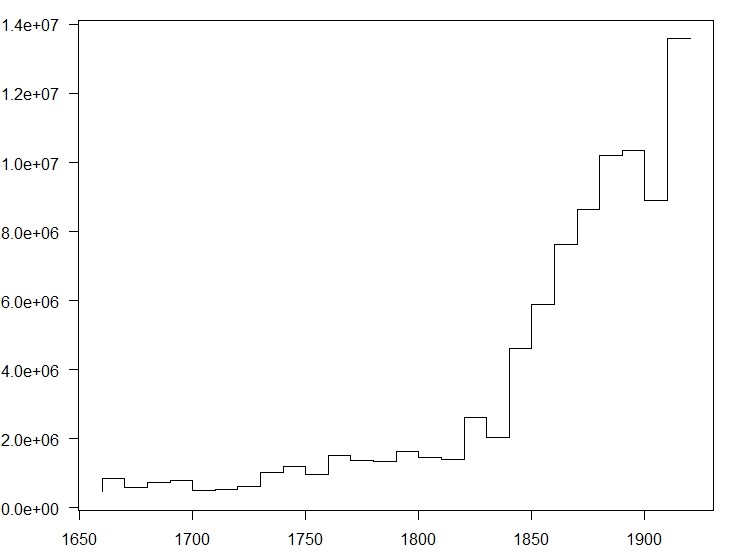
As a corpus we use a portion of the Royal Society Corpus (release 5.1), ranging from 1665 to 1929. The corpus comprises 91.2 Mio tokens over about 462.000 types and has been split into 27 decades, with the number of tokens ranging between 455.351 and 13.583.475. For a more detailed breakdown see Figure 1. The raw frequencies per decade are available in decFreq1929.zip.
Word Embeddings
For computing word embeddings we use word2vec skipgrams (Mikolov) and structured skipgrams introduced by (Ling et al). Whereas skipgrams represent the left/right usage context of a word as a bag of words, structured skipgrams represent each position of the context separately. For characterizing content words skipgrams and structured skipgrams seem to fare equally well, but structured skipgrams do a better job for characterizing function words.
For computing period specific word embeddings that are aligned with each other, we use two variatiants of the approach of Dubossarsky et al. (2015), Fankhauser and Kupietz (2017). Training for the first period is either initialized randomly (noinit) or with embeddings for the complete corpus (init). All subsequent periods are initialized with the embedding of their previous period. For the noinit option, embeddings for the complete corpus are initialized with embeddings for the last period. With random initialization low frequency words tend to be rather arbitrarily concentrated in the center of the semantic space for the first one or two periods. This is avoided with corpus initialization, however, the positioning of low frequency words may not really reflect their actual usage during the first few periods.
Table 1 lists all variants of embeddings currently available. Column Init distinguishes between corpus initialization and random initialization. Column Train Counts says whether training uses period specific word counts (yes) or the word counts for the complete corpus (no). Using period specific word counts is the more sensible approach, because it properly anneals the learning rate alpha and draws negative samples according to period specific counts rather than corpus wide ones. The original diachronic visualizations, however, have used corpus wide counts, and are included here for comparability. Column Architecture distinguishes between structured skipgrams (recommended) and skipgrams. For all visualizations the underlying embeddings are also available for download.
| Rec | Init | Train Counts | Architecture | Visualization | Vectors |
|---|---|---|---|---|---|
| yes | no | struct skip | rsc-init-tc0-t3 | rsc-vectors-init-tc0-t3.zip | |
| no | no | struct skip | rsc-noinit-tc0-t3 | rsc-vectors-noinit-tc0-t3.zip | |
| X | yes | yes | struct skip | rsc-init-tc1-t3 | rsc-vectors-init-tc1-t3.zip |
| X | no | yes | struct skip | rsc-noinit-tc1-t3 | rsc-vectors-noinit-tc1-t3.zip |
| yes | no | skipgram | rsc-init-tc0-t1 | rsc-vectors-init-tc0-t1.zip | |
| no | no | skipgram | rsc-noinit-tc0-t1 | rsc-vectors-noinit-tc0-t1.zip | |
| yes | yes | skipgram | init-tc1-t1 | rsc-vectors-init-tc1-t1.zip | |
| no | yes | skipgram | noinit-tc1-t1 | rsc-vectors-noinit-tc1-t1.zip |
All embeddings use a hidden layer with dimension 100, a window size of +/-5, negative sampling 10, and a minimum frequency of 5 in the complete corpus. Period specific word embeddings have been trained with 25 iterations, corpus embeddings with 5.
Visualization
The visualization consists of four main components:
(1) Bubble Chart
To the left, a bubble chart represents the color encoded semantic space of words, with the size of bubbles proportional to the square root of the relative frequency in the chosen period, and the color indicating the slope of the diachronic growth of a word or the period with its maximum relative frequency. Words can be clicked for further analysis.
(2) Line Chart
To the top right frequency change of individual words is represented by simple line charts showing the fitted 2nd order polynomials of the logit transformed relative frequencies. The line chart also doubles as a selector for individual periods.
(3) Options
The top right also provides a number of visualization options. The first group of options applies to the bubble chart:
- +/- zooms the visualization in and out as an alternative to zooming with the scroll wheel.
- </> moves to the next (previous) period.
- ? brings up this page.
- Zoom chooses between different ways to determine which words are shown on different zoom levels (ranging from 0 to 14). With freq clst and kld clst zoom levels are computed by partitioning the words into an increasing number of clusters (from 200 to 30.000) and assigning only the most frequent (freq clst) or most typical (kld clst) word of each cluster to a zoom level. This approach distributes the bubbles rather evenly in the semantic space. In contrast, freq and kld simply associate the top 200 words to the first zoom level and so on. This leads to more unevenly distributed bubbles, but shows more clearly which regions are mainly populated by a period.
- Color chooses between coloring the bubbles by the slope of their growth vs. their period with maximum relative frequency.
- Show chooses between displaying bubbles and words, bubbles only, and words only.
- Traject chooses between displaying a trajectory of the currently selected word's semantic position over time or not.
- Graph chooses between graphing the growth of a word in frequency per million or logit of frequency per million, or its paradigmatic productivity over time.
- Show chooses between showing points and fitted lines, fitted lines only, or fitted lines only.
- Fit chooses between fitting a polynomial of degree 2 or of degree 1.
- Clear chart clears the chart and currently selected words. Graphs for individual words can be discarded by clicking on their legend in the line chart.
The last two buttons are for choosing the number of more zoom levels to show for bubbles (just a convenience option for producing pretty pictures), and choosing whether the word table should reload on demand or always (default: on demand).
(4) Word Table
The bottom right provides a word list for the chosen period, with the following columns:
- word gives the word.
- fpm its frequency per million in the period.
- kld its typicality in comparison to the complete corpus. For the complete corpus it gives the average typicality in comparison to all periods.
- kldp its typicality in comparison to the previous period, for the first period its typicality in comparison to the last period, and for the complete corpus the average kldp.
- ent its paradigmatic productivity in the period or complete corpus.
- entd the slope of the paradigmatic productivity over time.
- dist the cosine distance between period specific embedding and the corpus embedding. For the complete corpus it gives the maximum distance to some period. The distance is multiplied by the sign of its typicality.
- decs the number of periods in which the word occurs at least once. This is mainly useful for filtering out words which occur in only few periods (e.g. < 15 or 20), and thus have now representative slope in paradigmatc productivity.
The word list can be sorted on all columns, searched for words, and filtered by giving lower bounds. Filtering and sorting is in particular useful to focus on words with a minimum frequency per million, on words typical for a period (kld > 0), or for looking for words with a high slope in productivity. Clicking on a word zooms and centers the bubble chart on its position in the chosen period.
References
tbd