Measuring and Visualizing Diachronic Word Use
Summary
This visualization extends the original diachronic visualization with a variety of measures to analyse word use along the lines of the domain specific visualization. Currently the following measures are supported:
- Typicality of a word measures how typical a word is for a time period compared to another time period. Informally, if a word is significantly more frequent in a period, it is typical for the period.
- Paradigmatic Productivity of a word measures how many (paradigmatically) similar words are used in a period. A word w with a paradigmatic neighbourhood (semantic field) consisting of many words is considered highly productive 2.
- Syntagmatic Productivity of a word measures how many different words occur in the syntagmatic context of the word 3.
- Ambiguity of a word measures how different its use in one period is from another. Formally, this is defined as the cosine distance between the period specific embeddings and the corpus embedding of a word.
Corpus
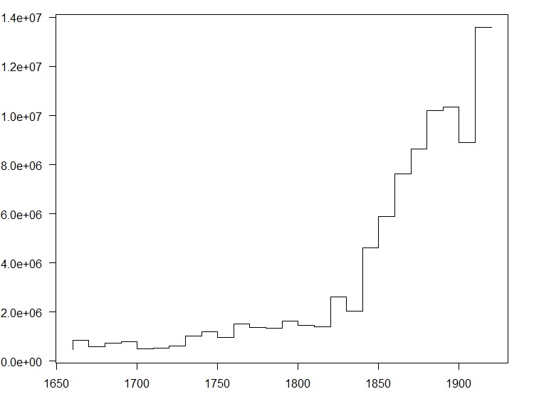
As a corpus we use a portion of the Royal Society Corpus (release 5.1), ranging from 1665 to 1929. The corpus comprises 91.2 Mio tokens over about 462.000 types and has been split into 27 decades, with the number of tokens ranging between 455.351 and 13.583.475. For a more detailed breakdown see Figure 1. The raw frequencies per decade are available in decFreq1929.zip, decFreq1929Pos.zip.
Word Embeddings
For computing word embeddings we use word2vec skipgrams (Mikolov et al. 2013) and structured skipgrams introduced by Ling et al. (2015). Whereas skipgrams represent the left/right usage context of a word as a bag of words, structured skipgrams represent each position in the context separately. For characterizing content words skipgrams and structured skipgrams seem to fare equally well, but structured skipgrams do a better job for characterizing function words.
For computing period specific word embeddings that are aligned with each other, we use two variants of the approach of Dubossarsky et al. (2015), Fankhauser and Kupietz (2017). Training for the first period is either initialized randomly (noinit) or with embeddings for the complete corpus (init). All subsequent periods are initialized with the embeddings of their previous period. For the noinit option, embeddings for the complete corpus are initialized with embeddings for the last period.
For words with enough support these two variants seem fairly equivalent. However, low frequency words can behave rather differently: With random initialization (noinit) low frequency words tend to be rather arbitrarily concentrated in the center of the semantic space for the first few periods. Corpus initialization (init) avoids this, but then the positioning of low frequency words may not really reflect their actual usage during the first few periods. Likewise, noinit may bias the representation of low frequency words for the complete corpus by the representation of the last period. Moreover, noinit also leads to partially erratic movement in the semantic space over time, evident by a larger average distance of word embeddings over time.
Altogether, option init together with carefully considering/filtering out low frequency words is recommended as default 5.
Table 1 lists all variants of embeddings currently available. Column Init distinguishes between corpus initialization and random initialization. Column Train Counts says whether training uses period specific word counts (yes) or the word counts for the complete corpus (no). Using period specific word counts is the more sensible approach, because it properly anneals the learning rate alpha and draws negative samples according to period specific counts rather than corpus wide ones. The original diachronic visualizations, however, have used corpus wide counts, and are included here for comparability. Column Architecture distinguishes between structured skipgrams (recommended) and skipgrams. For the two recommended options there are also embeddings available with part-of-speech attached to words (Column PoS). For all visualizations the underlying embeddings are also available for download.
| Rec | PoS | Init | Train Counts | Architecture | Visualization | Vectors |
|---|---|---|---|---|---|---|
| *** | no | yes | yes | struct skip | rsc-init-tc1-t3 | rsc-vectors-init-tc1-t3.zip |
| * | no | no | yes | struct skip | rsc-noinit-tc1-t3 | rsc-vectors-noinit-tc1-t3.zip |
| *** | yes | yes | yes | struct skip | rsc-pos-init-tc1-t3 | rsc-vectors-pos-init-tc1-t3.zip |
| * | yes | no | yes | struct skip | rsc-pos-noinit-tc1-t3 | rsc-vectors-pos-noinit-tc1-t3.zip |
| no | yes | no | struct skip | rsc-init-tc0-t3 | rsc-vectors-init-tc0-t3.zip | |
| no | no | no | struct skip | rsc-noinit-tc0-t3 | rsc-vectors-noinit-tc0-t3.zip | |
| no | yes | yes | skipgram | init-tc1-t1 | rsc-vectors-init-tc1-t1.zip | |
| no | no | yes | skipgram | rsc-noinit-tc1-t1 | rsc-vectors-noinit-tc1-t1.zip | |
| no | yes | no | skipgram | rsc-init-tc0-t1 | rsc-vectors-init-tc0-t1.zip | |
| no | no | no | skipgram | rsc-noinit-tc0-t1 | rsc-vectors-noinit-tc0-t1.zip |
All embeddings use a hidden layer with dimension 100, a window size of +/-5, negative sampling 10, and a minimum frequency of 5 in the complete corpus. Period specific word embeddings have been trained with 25 iterations, corpus embeddings with 5.
In addition, there is also a visualization of the Spiegel/Zeit-Corpus available. This is based on embeddings with a hidden layer with dimension 200.
Visualization
The visualization consists of four main components:
(1) Bubble Chart
To the left, a bubble chart represents the color encoded semantic space of words, with the size of bubbles proportional to the square root of the relative frequency in the chosen period, and the color indicating the slope of the diachronic growth of a word or the period with its maximum relative frequency. Words can be clicked for further analysis.
(2) Line Chart
To the top right frequency change of individual words is represented by simple line charts showing the fitted 2nd order polynomials of the logit transformed relative frequencies. The line chart also doubles as a selector for individual periods.
(3) Options
The top right also provides a number of visualization options. The first group of options applies to the bubble chart:
- +/- zooms the visualization in and out as an alternative to zooming with the scroll wheel.
- </> moves to the next (previous) period.
- ? brings up this page.
- Zoom chooses between different ways to determine which words are shown on different zoom levels (ranging from 0 to 14). With freq clst and kld clst zoom levels are computed by partitioning the words into an increasing number of clusters (from 200 to 30.000) and assigning only the most frequent (freq clst) or most typical (kld clst) word of each cluster to a zoom level. This approach distributes the bubbles rather evenly in the semantic space. In contrast, freq and kld simply associate the top 200 words to the first zoom level and so on. This leads to more unevenly distributed bubbles, but shows more clearly which regions are mainly populated by a period.
- Color chooses between coloring the bubbles by the slope of their growth vs. their period with maximum relative frequency.
- Show chooses between displaying bubbles and words, bubbles only, and words only.
- Traject chooses between displaying a trajectory of the currently selected word's semantic position over time or not.
- Graph chooses between graphing the growth of a word in frequency per million or logit of frequency per million, or its paradigmatic productivity over time.
- Show chooses between showing points and fitted lines, fitted lines only, or fitted lines only.
- Fit chooses between fitting a polynomial of degree 2 or of degree 1.
- Clear chart clears the chart and currently selected words. Graphs for individual words can be discarded by clicking on their legend in the line chart.
The last two buttons are for choosing the number of more zoom levels to show for bubbles (just a convenience option for producing pretty pictures), and choosing whether the word table should reload on demand or always (default: on demand). Clicking on the y-axis toggles between absolute and relative scaling.
(4) Word Table
The bottom right provides a word list for the chosen period, with the following columns:
- word gives the word.
- fpm its frequency per million in the period.
- kld its typicality in comparison to the complete corpus. For the complete corpus it gives the average typicality in comparison to all periods.
- kldp its typicality in comparison to the previous period, for the first period its typicality in comparison to the last period, and for the complete corpus the average kldp
- pprod its paradigmatic productivity in the period or complete corpus.
- pprodΔ the slope of the paradigmatic productivity over time for the complete corpus, and the difference between corpus paradigmatic productivity and period pprod.
- sprod its syntagmatic productivity in the period or complete corpus.
- sprodΔ the slope of the syntagmatic productivity over time for the complete corpus, and the difference between corpus syntagmatic productivity and period sprod.
- dist the cosine distance between period specific embedding and the corpus embedding. For the complete corpus it gives the maximum distance to some period. The distance is multiplied by the sign of its typicality for sorting.
- decs the number of periods in which the word occurs at least once. This is mainly useful for filtering out words which occur in only few periods (e.g. < 15 or 20), and thus have no representative slope in productivity.
The word list can be sorted on all columns, searched for words, and filtered by giving lower bounds. Filtering and sorting is in particular useful to focus on words with a minimum frequency per million, on words typical for a period (kld > 0), or for looking for words with a high slope in productivity. Clicking on a word zooms and centers the bubble chart on its position in the chosen period.
Macro Analysis
Measures over Time
Figure 2 breaks down productivity by (some) Part-of-Speech. As a general trend, paradigmatic productivity decreases consistently, whereas syntagmatic productivity increases. Nouns NN, verbs VV, and adjectives JJ behave very similar in diachronic productivity, however the overall trends are more pronounced for verbs. In particular, verbs start out with higher paradigmatic productivity than nouns and end up with a lower one. Adverbs RB have generally a lower paradigmatic and higher syntagmatic productivity than the average. Finally, determiners (like other function words) have unsurprisingly significantly higher syntagmatic productivity, and their diachronic development in paradigmatic productivity is much more erratic. Whereas Figure 2 (a,b) considers all words with minimum frequency 50 in the corpus (after discarding numbers etc.), Figure 2 (c,d) considers only words occuring in all decades, to account for the dominance of the corpus by later periods. As can be seen, the general trends in productity over time remain. All values are computed as type based means. Averaging over each individual token occurrence corroborates the overall trend of decreasing paradigmatic productivity, whereas syntagmatic productivity per token also decreases slightly.
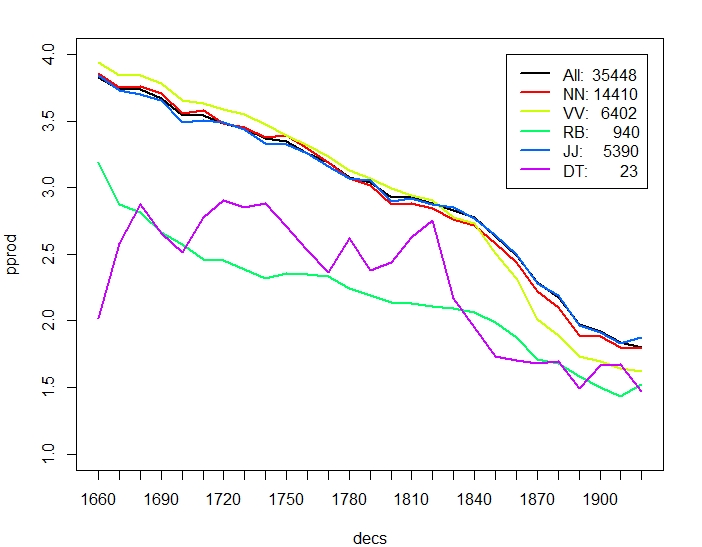
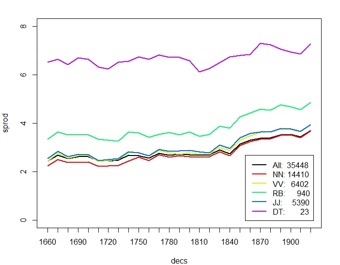
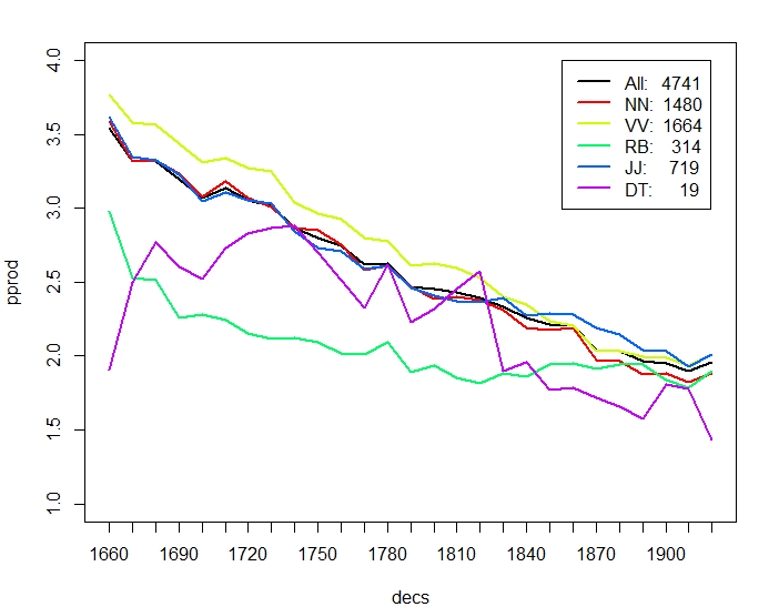
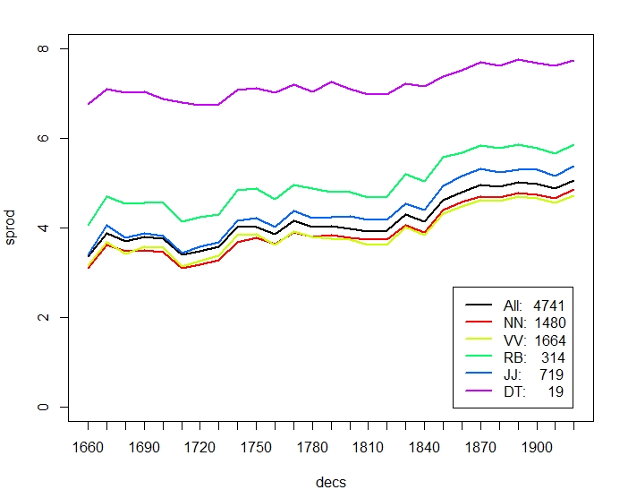
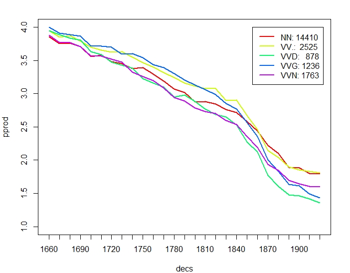
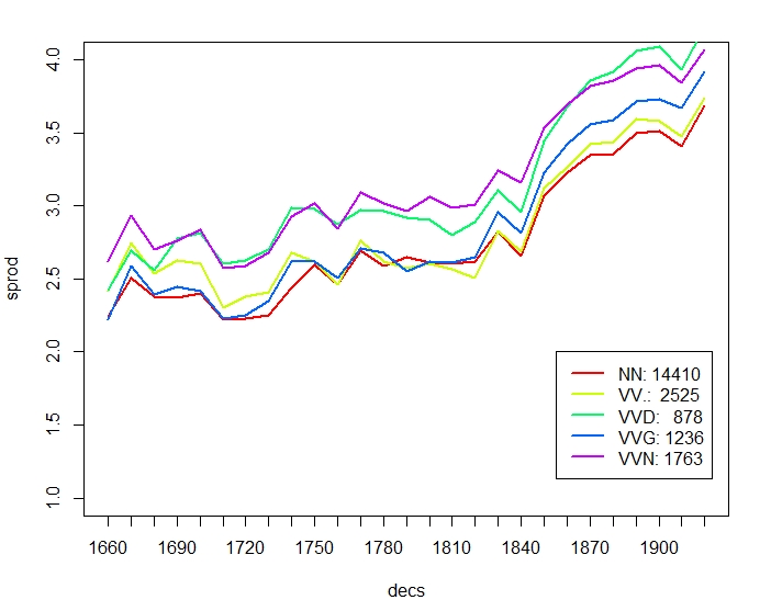
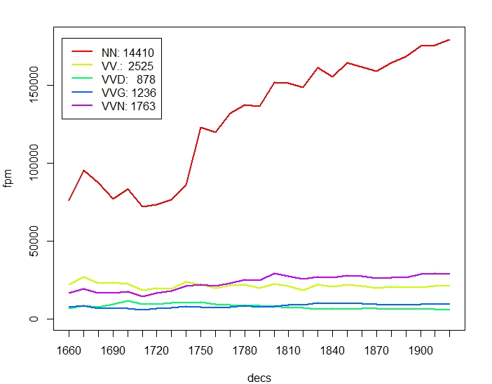
Figure 3 compares productivity over time between nouns and individual verb classes. The overall trend of verbs decreasing more strongly than nouns in paradigmatic productivity is mainly due to participles (VVG present participle, VVN past participle) and past tense, VVD, which may sometimes be mixed up with VVN. Base form VV and present tense VVZ, VVP show a less pronounced difference to NN. Likewise, participles in general have higher syntagmatic productivity than nouns. In terms of overall increase of relative frequency, nouns stand out by more than doubling over time, but also participles increase by almost 75% (VVN) and 25% (VVG) over time.
Correlations
With few exceptions, the introduced measures are largely orthogonal, i.e., they are basically uncorrelated. Table 2 (a) gives the Spearman rank correlations between the measures for the complete corpus. As to be expected by construction 1, there exists a weak positive correlation between frequency per million and typicality; in this case the Pearson correlation is much more pronounced (0.8). There also exists a weak positive correlation between frequency and syntagmatic productivity, i.e., higher frequency words (function words) tend to occur in more different contexts. Conversely, frequency and paradigmatic productivity are negatively correlated, and indeed low frequency words tend to have slightly more paradigmatic neighbours. These correlations are rather robust over different settings (with/without initialization, with/without PoS taggings).
| fpm | typ | pprod | sprod | dist | |
|---|---|---|---|---|---|
| fpm | 1.00 | 0.46 | -0.48 | 0.43 | -0.26 |
| typ | 0.46 | 1.00 | -0.20 | 0.22 | 0.04 |
| pprod | -0.48 | -0.20 | 1.00 | -0.26 | 0.08 |
| sprod | 0.43 | 0.22 | -0.26 | 1.00 | -0.02 |
| dist | -0.26 | 0.04 | 0.08 | -0.02 | 1.00 |
| Mean | 166.52 | 56.60 | 3.18 | 6.00 | 0.28 |
| StD | 1757.58 | 524.76 | 0.68 | 1.15 | 0.06 |
| fpm | dist | fpmΔ | pprodΔ | sprodΔ | |
|---|---|---|---|---|---|
| fpm | 1.00 | -0.26 | 0.58 | 0.64 | 0.19 |
| dist | -0.26 | 1.00 | -0.09 | -0.38 | 0.05 |
| fpmΔ | 0.58 | -0.09 | 1.00 | 0.29 | 0.72 |
| pprodΔ | 0.64 | -0.38 | 0.29 | 1.00 | 0.05 |
| sprodΔ | 0.19 | 0.05 | 0.72 | 0.05 | 1.00 |
| Mean | 166.52 | 0.28 | -0.56 | -2.63 | 2.38 |
| StD | 1757.58 | 0.06 | 2.83 | 2.27 | 2.05 |
Table 2 (b) gives the Spearman rank correlations for the slopes of frequency, paradigmatic productivity, and syntagmatic productivity, taking only into account words that occur in all periods, and thus have rather reliable estimates for the slopes. The positive correlation of fpm (of the complete corpus) and fpmΔ just reflects the fact that the late periods have orders of magnitude more tokens than early periods. Thus words with high fpms also typically have high fpms during late periods, and thus a positive slope fpmΔ. However, the mean slope is roughly zero (larger standard deviation than mean). In contrast paradigmatic entropy has a significantly negative mean slope, and syntagmatic entropy a significantly positive mean slope. This indicates a general trend of expressing more diverse syntagmatic contexts with fewer paradigmatic choices. Interestingly, the positive correlation between fpm and sprod also shows as a rather strong positive correlation of the slopes fpmΔ and sprodΔ, whereas the negative correlation between fpm and pprod does not translate to a negative correlation of the respective slopes. However, the slope pprodΔ is positively correlated with fpm, i.e., higher frequency words tend to increase in paradigmatic productivity over time. Finally, there is a weak negative correlation between pprodΔ and the (maximum) distance of a word in the complete corpus and one of the individual periods, indicating that words with increasing paradigmatic productivity tend to be rather stable in their meaning.
(tbd) From previous analysis we know that close paradigmatic neighbours typically also have highly correlated fpmΔ. An open question then is, whether this also holds for productivity.
Micro Analysis
The visualization supports two main paths to finding possibly interesting diachronic developments in word use: Spot patterns and sort&filter. In the following we will illustrate these two by way of some example analyses. Unless explicitly stated otherwise all analyses are carried out on the embeddings with initialization.
Spot Patterns
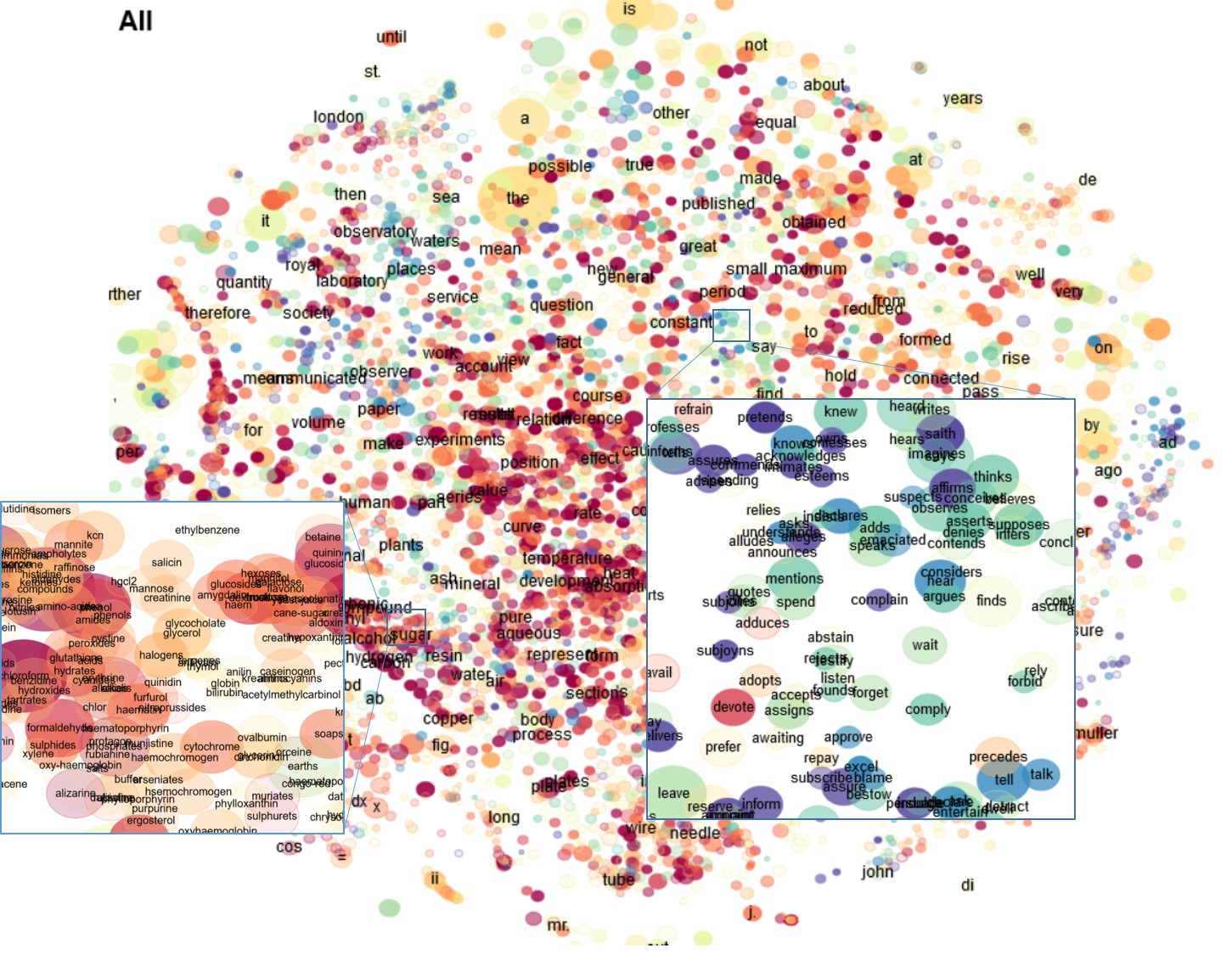
The bubbles overview allows to identify and zoom to paradigmatic clusters typical for a period, or more precisely, rising or falling fairly consistently. On the complete corpus (All) these clusters show as regions with a dominant color (blueish for falling, readish for rising). Figure 4 (a) shows two example clusters, a rising one with chemical compounds, and a falling one with communicative verbs in present tense.
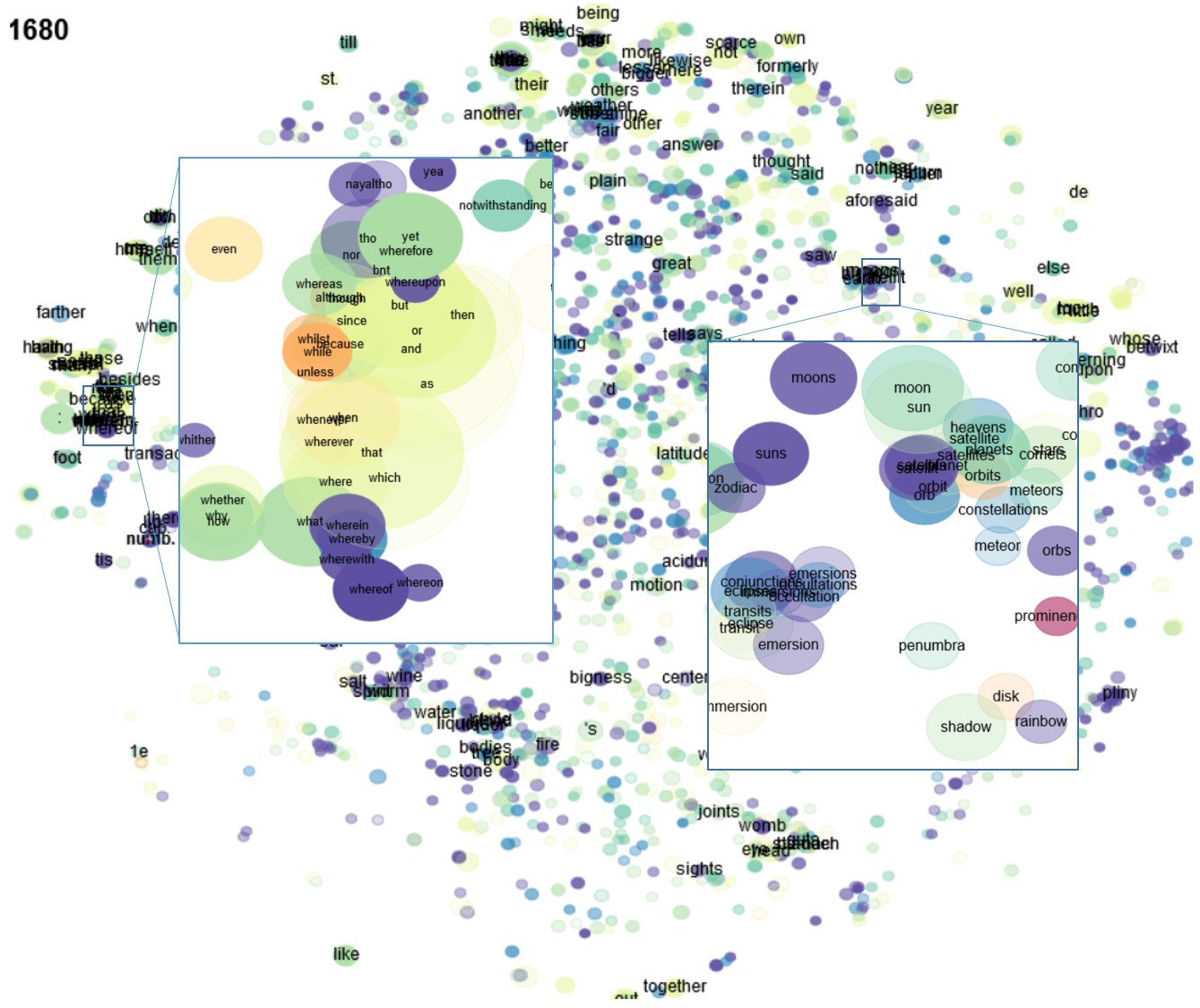
Because the corpus is dominated by late periods, falling clusters are less visible than rising clusters. These clusters can be more easily identified by selecting a particular period, preferably with option zoom: kld rather than zoom: freq clst to show the most typical words for a period. For example, Figure 4 (b) shows two falling paradigmatic clusters in 1680-89, one grammatical (of wh-adverbs) and one thematic (solar system).
Sort&Filter
Sorting (usually in decending order) is a simple means to identify possibly characteristic words for a particular decade or in diachronic change. For example Table 3 (a) lists the 10 most typical words in comparison with the complete corpus (kld) over time in steps of 50 years. The first three decades are dominated by (personal) pronouns and conjunctions indicating a personal reporting style (letters to the editor), the second three periods by rather generic thematic words (and symbols). The last column gives the average typicality of words in the complete corpus compared to individual periods. These clearly indicate the nominal style of the frequency wise dominant later periods. Table 3 (b) shows that the transition from personal reporting style to nominal style is rather continous: When comparing a decade with its immediately preceding decade, the most typical words in the first three decades overlap very much with the most typical words for the complete corpus. Again the second three decades, where the nominal style has settled in, are characterized by generic thematic words.
| 1670 | 1720 | 1770 | 1820 | 1870 | 1920 | All |
|---|---|---|---|---|---|---|
| , | i | , | i | ; | ) | the |
| he | 'd | i | needle | w. | ( | ; |
| hath | it | ditto | observations | e. | is | of |
| that | 's | it | inches | on | for | ) |
| they | they | air | mean | 8vo | vol. | ( |
| : | pox | 's | r | \amp | in | in |
| them | them | wind | magnets | n. | p. | is |
| and | or | quicksilver | grains | s | per | a |
| it | he | them | : | sea | values | on |
| some | aequator | will | distance | fathoms | the | and |
| 1670 | 1720 | 1770 | 1820 | 1870 | 1920 | All |
|---|---|---|---|---|---|---|
| , | , | the | needle | ; | ( | the |
| of | the | , | ; | \amp | ) | of |
| the | of | in | at | 8vo | the | , |
| and | to | is | mean | \apos | of | ) |
| in | will | of | magnets | w. | and | ( |
| ; | be | a | time | s | a | ; |
| a | a | it | inches | e. | is | in |
| which | in | ; | obs. | \lt | for | is |
| to | force | and | nerve | on | golgi | vol. |
| that | aequator | ditto | observations | \gt | fig. | a |
Finally, Table 4 looks at (a) paradigmatic and (b) syntagmatic productivity: To have enough datapoints for estimating the slope in productivity, here we consider only words occurring in at least 20 out of 27 decades, with a minimum frequency per million 100, and we filter out non alphabetic words (by the regular expression ^[A-Za-z]+$ in the search field for column word). In absolute terms, named entities (and numbers)6 have the highest paradigmatic productivity (pprod↓). They tend to occur in rather regular contexts and they constitute a very open class In contrast, closed class function words (pprod↑ sorted in ascending order) have low paradigmatic productivity. In terms of change over time, (pprodΔ↓) adverbs used for construing discourse stand out with increasing paradigmatic productivity. The list of words with decreasing paradigmatic productivity seems a bit arbitrary though, but then just looking at the top 10 words does not always suffice.
| pprod↓ | pprodΔ↓ | pprod↑ | pprodΔ↑ |
|---|---|---|---|
| june | consequently | of | contact |
| july | thus | the | distribution |
| usually | still | alone | to |
| april | rather | our | group |
| march | again | per | of |
| january | however | those | active |
| soon | probably | any | independent |
| apparently | completely | for | unit |
| entirely | even | its | you |
| completely | air | to | standard |
| sprod↓ | sprodΔ↓ | sprod↑ | sprodΔ↑ |
|---|---|---|---|
| des | completely | however | however |
| de | previously | presence | hand |
| der | j | existence | said |
| j | rapidly | regarded | indeed |
| being | gas | regard | author |
| or | group | roy | course |
| were | arrangement | addition | think |
| was | der | top | do |
| et | average | bottom | due |
| of | apparently | royal | communicated |
The words with the highest syntagmatic productivity (Table 4 (b) sprod↓) are mostly function words, corroborating the analysis (DT) in Figure 2. The words with the lowest syntagmatic productivity sprod↑ appear to be words which occur mostly in rather fixed contexts (in existence, presence, with regard to, ...). Words with increasing syntagmatic productivity sprodΔ↓ comprise adverbs but also generic nouns with presumably many different modifiers (gas). Finally, words with decreasing syntagmatic productivity sprodΔ↑ indicate words increasingly becoming used in rather fixed context (e.g. due to, other hand, do not).
Further Reading
For more information see Bizzoni et al. 2020 and Teich et al. 2021.
Footnotes
- Typicality of a word \(x\) is defined as its contribution to the Kullback-Leibler Divergence between the (unigram) language model of a period (or more generally corpus) \(D_1\) to the language model of another period \(D_2\), also called relative entropy: \[Typ(x,D_1,D_2) = p(x|D_1) log(p(x|D_1)/p(x|D_2))\] This gives the number of bits lost when encoding \(x\) with an optimal encoding for \(D_2\) instead of \(D_1\). (see also: Contrastive Analysis)
- Paradigmatic Productivty is measured by the entropy over all close paradigmatic neighbours \(x_i\) of a word \(x\), including \(x\): \[ParProd(x)=-\sum_{cos(x_i,x) \gt \theta} p(x_i|C_x) log(p(x_i|C_x))\] \[\textrm{with}\:p(x_i|C_x) = \frac{cos(x_i,x) freq(x_i)}{\sum_{x_j}cos(x_j,x)freq(x_j)}\] i.e., \(P(x_i|C_x)\) is the conditional probability of word \(x_i\) in the close neighbourhood of word \(x\), weighted by the cosine similarity between \(x_i\) and \(x\) (max 25 words, cosine similarity \(\gt \theta = 0.6\)). For the chosen parameters this measure ranges between 0, no neighbours and \(log(25) = 4.64\), all 25 neighbours with maximum similartiy 1, uniformly distributed. Note that the term productivity is borrowed from analysis of word formation. Pexman et al. (2008) employ a closely related measure - number of paradigmatic neighbours - as an aspect of semantic richness.
- Syntagmatic Productivity is measured by the entropy over all syntagmatic neighbours of a word \(x\) within a window \(C_x\) of +/- 1: \[SynProd(x)=-\sum_{c_i \in C_x} p(c_i|x) log(p(c_i|x))\] \[\textrm{with}\: C_x = \{x_{-1}|x_{-1},x\} \cup \{x_1|x,x_1\}\] We have also looked at syntagmatic productivity in the window +/- 3, and the corresponding left and right only windows. All these windows result in highly correlated productivities (\(\gt 0.9\) spearman and pearson) with the chosen window.
- Other measures for ambiguity exist, such as curvature aka clustering coefficient (Dorow et al. 2005). Moreover, there exist more sophisticated approaches to analyse and detect ambiguity via word embeddings, for an overview see e.g. Van Landeghem (2016).
- We get rather convincing correlations \(\gt 0.7\) on all measures between init and noinit options for words with \(fpm(x) > 10\) in the complete corpus.
- Incidentally, foreign words occurring in stretches of text in foreign language also have an artificially high paradigmatic productivity: They are simply considered as one close knit neighbourhood of aliens.
Contact
Peter Fankhauser fankhauser at ids-mannheim.de
References
- Bizzoni, Y., Degaetano-Ortlieb, S., Fankhauser, P., Teich, E. (2020). Linguistic Variation and Change in 250 Years of English Scientific Writing: A Data-Driven Approach. In: Frontiers in Artificial Intelligence, Vol. 3. doi: 10.3389/frai.2020.00073.
- Dorow, B., Widdows, D., Ling K., Eckmann, J-P., Sergi, D., Moses, E. (2005). Using Curvature and Markov Clustering in Graphs for Lexical Acquisition and Word Sense Discrimination. In MEANING-2005, 2nd Workshop organized by the MEANING Project, February 3rd-4th 2005, Trento, Italy
- Dubossarsky, H., Tsvetkov, Y., Dyer, C., Grossman, E. (2015). A bottom up approach to category mapping and meaning change. In Pirrelli, Marzi & Ferro (eds.), Word Structure and Word Usage. Proceedings of the NetWordS Final Conference.
- Peter Fankhauser and Marc Kupietz (2017) Visualizing Language Change in a Corpus of Contemporary German. Corpus Linguistics Conference 2017.
- Ling, W., Dyer, C., Black, A., & Trancoso, I. (2015). Two/too simple adaptations of word2vec for syntax problems. In Proc. of NAACL.
- Mikolov, T., Sutskever, I., Chen, K., Corrado, G. S., Dean, J. (2013). Distributed representations of words and phrases and their compositionality. In Proceedings of NIPS 2013, 3111–3119.
- Pexman P.M., I.S. Hargreaves, P.D. Siakaluk, G.E. Bodner, J. Pope (2008). There are many ways to be rich: effects of three measures of semantic richness on visual word recognition. Psychon Bull Rev. 2008 Feb;15(1):161-7.
- Teich, E., Fankhauser, P., Degaetano-Ortlieb, S., Bizzoni, Y. (2021). Frontiers in Communication, Vol. 5. doi: 10.3389/fcomm.2020.620275.
- Van der Maaten, L. & Hinton, G. (2008). Visualizing Data using t-SNE. In Journal of Machine Learning Research 1, 1-48.